3.6 Interpolation and Approximation

Spline functions are useful for interpolating and approximating data or functions. Sh provides implementations of several basic spline types as well as evaluation of polynomials; see Table 3.11.

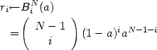
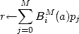
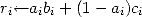
Linear interpolation is the most basic interpolation method supported, but Sh also supports Bézier and Hermite splines. Bézier splines can be evaluated either by first evaluating the Berenstein basis functions and then forming an affine combination of control points, or by calling one of the overloaded direct evaluation functions for each supported order. The cubic Hermite spline permits the interpolation of a pair of data points with specified tangents.

Evaluation of polynomials relative to the power basis is also supported, given a tuple of coefficients.

Operation   r a,b,c,... Description / bernstein<N>  N 1 Evaluation of the Bernstein (Bézier) basis functions of order M at parameter a: / bezier   N 1,N,N,... Bézier spline of degree M evaluated at parameter a using control points p0 = b, p1 = c, ...pM: / hermite   N 1,N,N,N,N Cubic Hermite spline evaluated at parameter a interpolating b at 0 with tangent c and d at 1 with tangent e. lerp   N N,N,N Linear interpolation lerp   N 1,N,N Linear interpolation with scalar promotion / poly   N N,M Evaluation of polynomial of order N at a using coefficients in b:   Table 3.11: Spline and polynomial functions.

Note: This manual is available as a bound book from AK Peters, including better formatting, in-depth examples, and about 200 pages not available on-line.